Descriptors
For the PDF version, click here
Amino Acid Composition
Amino Acid Composition (AAC)
The amino acid composition method (1) calculates the frequency of each natural amino acid in the sequence.
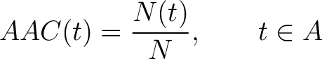
Where  is the group of the 20 natural amino acids,
  is the number of
times amino acid
is the number of
times amino acid  appears in the sequence, and
  is the sequence
length.
is the sequence
length.
- Vector length

- Parameters None
Dipeptide Composition (DPC)
The dipeptide composition method (1) calculates the frequency of each consecutive amino acid pair in the sequence.
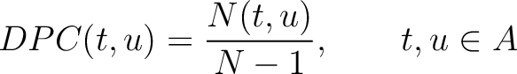
Where is the group of the 20 natural amino acids,  is the number
of times amino acid pair
is the number
of times amino acid pair  appears in the sequence, and is the sequence
length.
appears in the sequence, and is the sequence
length.
- Vector length

- Parameters None
Tripeptide Composition (TPC)
The tripeptide composition method (1) calculates the frequency of each consecutive amino acid triplet in the sequence.
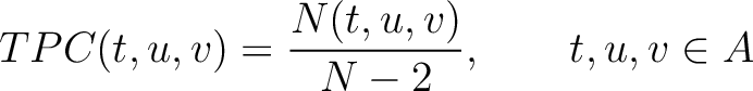
Where is the group of the 20 natural amino acids,
 is the number of times amino acid triplet
  appears in the
sequence, and is the sequence length.
appears in the
sequence, and is the sequence length.
- Vector length
- Parameters None
Composition of k-Spaced Amino Acid Pairs (CKSAAP)
The composition of k-spaced amino acid pairs method (2) calculates the
frequency of amino acid pairs separated by  characters.

Where is the group of the 20 natural amino acids, is the number
of times amino acid pair , separated by characters, appears
in the sequence, is the sequence length and  is the maximum
number of . Two consecutive characters are separated by
is the maximum
number of . Two consecutive characters are separated by  . If
. If  ,
then each possible pair would be calculated for
,
then each possible pair would be calculated for
 and 5.
- Vector length
- Parameters
-
- –gap , default
5
- –gap
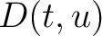
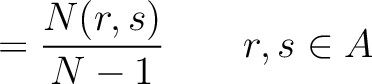
Dipeptide Deviation from Expected Mean (DDE)
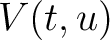
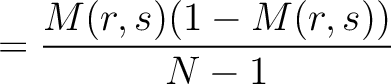
The dipeptide deviation from expected mean method (3) calculates the
dipeptide composition ( ), theoretical mean (
 ) and theoretical
variance (
) and theoretical
variance ( ) and applies the following formulas:
Where is the group of the 20 natural amino acids, is the number
of times the amino acid pair appears in the sequence,  and
and  are
the number of times the amino acid
are
the number of times the amino acid  or
or  appears in the
sequence, and is the sequence length.
appears in the
sequence, and is the sequence length.
- Vector length
- Parameters None
Amino Acid Pair Antigenicity Scale (AAPAS)
In the amino acid pair antigenicity scale method (4), for each existing amino acid pair, it counts the number of times they appear consecutively in the sequence and multiplies them by their normalized amino acid pair antigenicity scale, which can be understood as the chance each amino acid pair is associated with an epitope.

Where is the group of the 20 natural amino acids, is the number
of times the amino acid pair appears in the sequence and
 is the normalized amino acid pair antigenicity scale for the pair .
The values of are in Supplementary Material 2. They were calculated as follows:
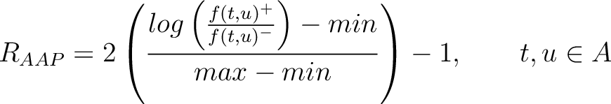
Where  and
and  are the frequencies of the amino acid pair in
the epitopes (obtained from the Bcipep database) (5) and non-epitopes (obtained
from the Swiss-Prot database) (6), respectively.
are the frequencies of the amino acid pair in
the epitopes (obtained from the Bcipep database) (5) and non-epitopes (obtained
from the Swiss-Prot database) (6), respectively.
- Vector length
- Parameters None
Composition Moment Vector (CMV)
The composition moment vector method (7) contains information of the position of each occurence for each amino acid in the sequence in its calculation.
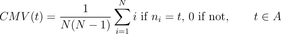
Where is the group of the 20 natural amino acids,  is the
  residue in the sequence and is the sequence length.
- Vector length
- Parameters None
Enhanced Amino Acid Composition (EAAC)
The enhanced amino acid composition method (8) calculates the frequency of each natural amino acid in a sliding window across the whole sequence.

Where is the group of the 20 natural amino acids,  is the
number of times amino acid appears in the sliding window
is the
number of times amino acid appears in the sliding window  and
and  is the
size of the sliding window. For example, the first sliding window
is the
size of the sliding window. For example, the first sliding window  would go from the
first amino acid
would go from the
first amino acid  to the amino acid
  , while the second
sliding window would go from the second amino acid
, while the second
sliding window would go from the second amino acid  to the amino acid
 .
.
- Vector length
- Parameters
-
- –window , default
5
- –window
- All sequences must have the same length
Grouped Amino Acid Composition
Grouped Amino Acid Composition (GAAC)
The grouped amino acid composition method (8) finds the proportion of each of the five group of proteins in the sequence. These five groups are based on their physicochemical properties, which are aliphatic (AGILMV), aromatic (FWY), positive (HKR), negative (DE) and uncharged (CNPQST) (9).
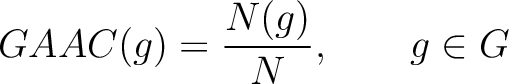
Where  are the 5 groups based on the amino acids' physicochemical properties,
  is
the number of times an amino acid belonging to the group
is
the number of times an amino acid belonging to the group  appears and is the
sequence length.
appears and is the
sequence length.
- Vector length

- Parameters None
Enhanced Grouped Amino Acid Composition (EGAAC)
The enhanced grouped amino acid composition method (8) finds the proportion of each of the five group of proteins in a sliding window across the peptide sequence. These five groups are based on their physicochemical properties, which are aliphatic (AGILMV), aromatic (FWY), positive (HKR), negative (DE) and uncharged (CNPQST) (9).

Where are the 5 groups based on the amino acids' physicochemical properties,  is the number of times an amino acid belonging to the group
appears in the sliding window and is the window size.
is the number of times an amino acid belonging to the group
appears in the sliding window and is the window size.
- Vector length
- Parameters
-
- –window , default
5
- –window
- All sequences must have the same length
Composition of k-Spaced Amino Acid Group Pairs (CKSAAGP)
The composition of k-spaced amino acid group pairs method (8) calculates the
frequency of amino acid pairs, grouped by their physicochemical properties as in GAAC, separated by
characters.

Where are the 5 groups based on the amino acids' physicochemical properties,  is the number of times amino acids from the groups
  , separated by
characters, are paired in the sequence, is the sequence
length and is the maximum number of . Two consecutive
characters are separated by . If , then each
possible pair would be calculated for
and 5.
, separated by
characters, are paired in the sequence, is the sequence
length and is the maximum number of . Two consecutive
characters are separated by . If , then each
possible pair would be calculated for
and 5.
- Vector length
- Parameters
-
- –gap , default
5
- –gap
Grouped Dipeptide Composition (GDPC)
The grouped dipeptide composition method (8) calculates the frequency of each consecutive amino acid group pair in the sequence.
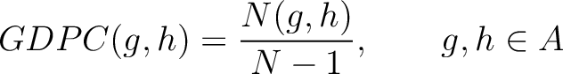
Where are the 5 groups based on the amino acids' physicochemical properties,
is the number of times amino acids from the groups appear
consecutively in the sequence, and is the sequence length.
- Vector length

- Parameters None
Grouped Tripeptide Composition (GTPC)
The grouped tripeptide composition method (8) calculates the frequency of each consecutive amino acid group triplet in the sequence.
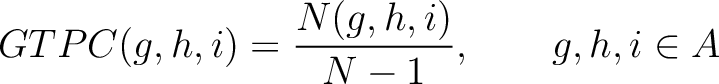
Where are the 5 groups based on the amino acids' physicochemical properties,
 is the number of times amino acids from the groups
  appear
consecutively in the sequence, and is the sequence length.
appear
consecutively in the sequence, and is the sequence length.
- Vector length

- Parameters None
Encoding Based on Grouped Weight (EBGW)
For the encoding based on grouped weight method (10), the amino acids are split in 4 groups, based on their hydrophobicity and charge:
- Neutral and non-polarity
-

- Neutral and polarity
-

- Acidic
- Basic
-
And then each amino acid would have an associated value for each group in the following way:

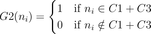
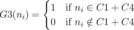
So, if an amino acid belongs to, for example, group  , then it would
pre-encode as 1 for the first group
, then it would
pre-encode as 1 for the first group  , and 0 for the other ones. If it belongs to group
  , it
would pre-encode as 1 for every group. This results in three binary sequences
, it
would pre-encode as 1 for every group. This results in three binary sequences  , one per group,
with
length, being the sequence length, and
, one per group,
with
length, being the sequence length, and  is a number between
1 and 3.
is a number between
1 and 3.

The full table associating amino acids with its group value can be found in Supplementary Material 2.
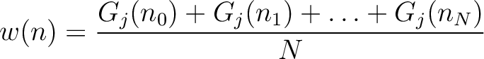
The normalized weight  of a characteristic sequence
  is the
frequency of 1 appearing in it.
is the
frequency of 1 appearing in it.
Given a number , the characteristic sequence can be split
into
subsequences. This way,
 represents a subsequence, where
 , and
, and
 is the largest integer below the result of the division inside.
Joining all values would yield the whole characteristic sequence. Hence,
is the largest integer below the result of the division inside.
Joining all values would yield the whole characteristic sequence. Hence,
 is the normalized weight of the subsequence
. This results in the following weight characteristic sequence:
is the normalized weight of the subsequence
. This results in the following weight characteristic sequence:

Finally, all three vectors (one per ) are concatenated.

- Vector length

- Parameters
-
- –k , default
30
- –k
Quasi-Sequence-Order
Both quasi-sequence-order and sequence-order-coupling number encodings (11) use the Grantham (12) and the Schneider-Wrede (13) distance matrices.
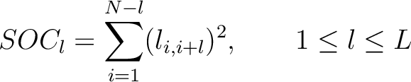
The  -th rank sequence-order-coupling number is a sum of squares of the distance (according
to the distance matrices) between two amino acids that are separated by characters in the
sequence.
-th rank sequence-order-coupling number is a sum of squares of the distance (according
to the distance matrices) between two amino acids that are separated by characters in the
sequence.
Where
 is the value in a distance matrix between two amino acids at positions
  and
and
 ,
,
 is
the maximum value of the lag value , and is the sequence
length.
is
the maximum value of the lag value , and is the sequence
length.
Sequence-Order-Coupling Number (SOCN)
This encoding is the concatenation of all  per distance
matrix.
per distance
matrix.
- Vector length

- Parameters
-
- –lag ,
default 30
- –lag
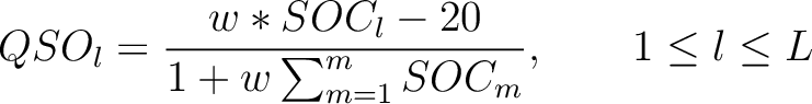
Quasi-Sequence-Order (QSO)
First, the quasi-sequence-order numbers for the amino acids must be calculated as follows:
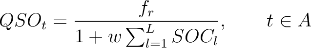
Where is the group of the 20 natural amino acids,  is the frequency
of each amino acid in the sequence (just as in AAC encoding), and
is the frequency
of each amino acid in the sequence (just as in AAC encoding), and  is a weight factor.
Then, the quasi-sequence-order numbers for the lag values must be calculated as follows:
Where is the group of the 20 natural amino acids, is the frequency
of each amino acid in the sequence (just as in AAC encoding), is a the lag value,
and
is a weight factor.
- Vector length
- Parameters
-
- –lag ,
default 30
- –weight ,
default 0.1
- –lag
Autocorrelation
The autocorrelation descriptors use the amino acid properties from the AAindex Database (14), found in the data/AAidx.txt file. The default indices used (CIDH920105, BHAR880101, CHAM820101, CHAM820102, CHOC760101, BIGC670101, CHAM810101, DAYM780201) were taken from the work by Xiao et al. (15). All the values in the indices are centralized and standardized for the autocorrelation encodings as follows:
Where is the group of the 20 natural amino acids,  is the value of
the property for the amino acid , and
is the value of
the property for the amino acid , and  and
and  are the average and standard deviation of all the 20 amino acids in the index, respectively.


Geary Autocorrelation (Geary)
The Geary autocorrelation (16) is calculated as:
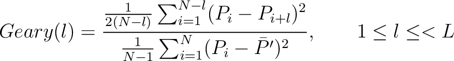
Where is the lag value, is the maximum lag
value,  and
and  are the centralized and standardized values for the amino acids
at positions and
are the centralized and standardized values for the amino acids
at positions and  , and
, and  is the
average property value between all amino acids in the sequence.
is the
average property value between all amino acids in the sequence.
- Vector length
 , where
  is the count of
used indices.
is the count of
used indices.
- Parameters
-
- –lag ,
default 30
- –indices
 ,
default 'CIDH920105, BHAR880101, CHAM820101, CHAM820102, CHOC760101, BIGC670101, CHAM810101,
DAYM780201' (
,
default 'CIDH920105, BHAR880101, CHAM820101, CHAM820102, CHOC760101, BIGC670101, CHAM810101,
DAYM780201' ( ).
).
- –lag
Moran Autocorrelation (Moran)
The Moran autocorrelation (17) is calculated as:
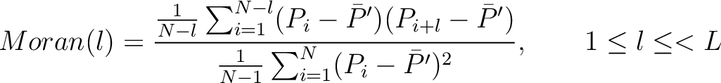
Where is the lag value, is the maximum lag
value, and are the centralized and standardized values for the amino acids
at positions and , and is the
average property value between all amino acids in the sequence.
- Vector length , where is the count of
used indices.
- Parameters
-
- –lag ,
default 30
- –indices ,
default 'CIDH920105, BHAR880101, CHAM820101, CHAM820102, CHOC760101, BIGC670101, CHAM810101,
DAYM780201' ().
- –lag
Normalized Moreau-Broto Autocorrelation (NMB)
The Normalized Moreau-Broto autocorrelation (18) is calculated as:
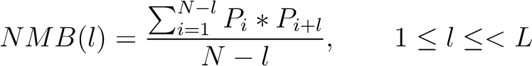
Where is the lag value, is the maximum lag
value, and and are the centralized and standardized values for the amino acids
at positions and .
- Vector length , where is the count of
used indices.
- Parameters
-
- –lag ,
default 30
- –indices ,
default 'CIDH920105, BHAR880101, CHAM820101, CHAM820102, CHOC760101, BIGC670101, CHAM810101,
DAYM780201' ().
- –lag
Composition/Transition/Distribution
The Composition/Transition/Distribution encodings (19), (20) are based on a categorical division of the 20 natural amino acids according to their structural and physicochemical properties. 13 properties were chosen on iFeature (8), and 1 (surface tension) was added (21), as listed in Supplementary Material 2.
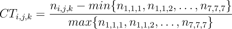
Composition (CTDC)
Calculates the frequency of each division per property.
Where  is the number of amino acids in the division
  found in the
sequence, and is the sequence length.
found in the
sequence, and is the sequence length.
- Vector length

- Parameters None
Transition (CTDT)
Calculates the frequency of each transition (division 1 to division 2, division 1 to division 3, etc.) per property between consecutive amino acids.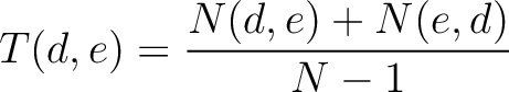
Where  and
and  are the numbers of consecutive amino acids from divisions and
 in
both orders (
in
both orders ( and
and  ), and is the sequence
length.
), and is the sequence
length.
- Vector length
- Parameters None
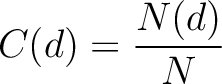
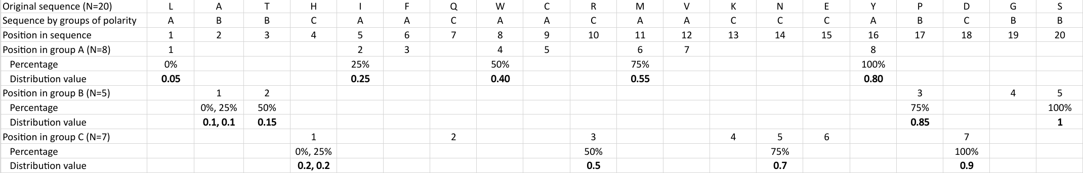
Distribution (CTDD)
Calculates where the first, 25%, 50%, 75% and 100% of amino acids in a division occur in a sequence. It is done
by highlighting all the amino acids that belong to a certain division in a sequence. Find the position of the
first occurence and divide it by (the sequence length). Then, find the position where the first 25%
(rounded down) of the amino acids in that division occurs in the sequence, and divide this position over . After
that, do the same with the other percentages (Figure 1).
 |


- Vector length

- Parameters None
Conjoint Triad
For the conjoint triad encodings, the amino acids were classified in 7 classes based on the dipoles and volumes
of the side chains (22):
 ,
,
 ,
,
 ,
,
 ,
,  ,
,  , and
, and  .
.
Conjoint Triad (CT)
The conjoint triad method (22) is calculated as:
Where  is the number of times three consecutive amino acids belonging to groups ,
and
are
seen in the sequence.
is the number of times three consecutive amino acids belonging to groups ,
and
are
seen in the sequence.
- Vector length

- Parameters None
k-Spaced Conjoint Triad (KSCT)
The k-Spaced conjoint triad method (8) is based on the conjoint triad method,
but instead of only evaluating consecutive amino acids, it evaluates triads separated by 0 to
characters. The original CT method is the same as KSCT with  .
.
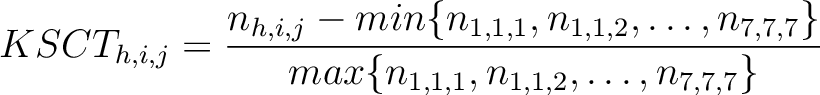
Where  is the number of times three consecutive amino acids belonging to groups
  ,
and
are
seen in the sequence. This should be evaluated for
,
and
are
seen in the sequence. This should be evaluated for
 , so it is calculated
  times. For
example, for , each triad is formed by the amino acids at positions ,
times. For
example, for , each triad is formed by the amino acids at positions ,  and
and
 for
for
 . For
. For  , each triad is
formed by the amino acids at positions , ,
, each triad is
formed by the amino acids at positions , ,  for
for
 . For
. For  , each triad is
formed by the amino acids at positions ,
, each triad is
formed by the amino acids at positions ,  ,
,  for
for
 .
.
- Vector length

- Parameters
-
- –k , default
1.
- –k
Pseudo-Amino Acid Composition
The pseudo-amino acid composition encodings use the hydrophobicity values proposed by Tanford (23), the hydrophilicity values proposed by Hopp and Woods (24) and the side chain mass values are the standard ones. Their initial values
are represented by  ,
,  and
and  , where is
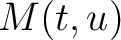
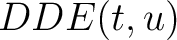
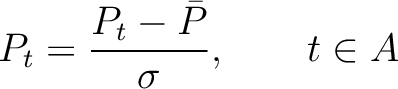
each of the 20 natural amino acids. These values are centralized and standardized as follows:
, where is
each of the 20 natural amino acids. These values are centralized and standardized as follows:
![$\displaystyle P(t) = \frac{
P^0(t) - \frac{1}{20}\sum_{i=1}^{20} P^0(i)
}{
\sqr...
...i=1}^{20}[P^0(i) - \frac{1}{20}\sum_{j=1}^{20}P^0(i)]^2}{20}}
}, \qquad t \in A$](/profeatx/static/profeatx/images/descriptors/img183.png)
Where is the group of the 20 natural amino acids, and  represents the
centralized and standardized value of any of the three properties (
represents the
centralized and standardized value of any of the three properties ( ,
,  ,
) of
the amino acid , so in the end we would have
,
) of
the amino acid , so in the end we would have  ,
,  and
and  .
.
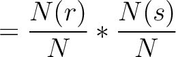
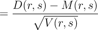
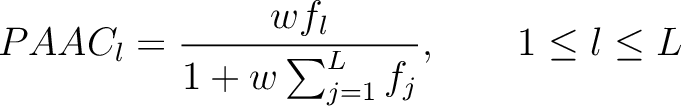
Pseudo-Amino Acid Composition (PAAC)
For the pseudo-amino acid composition method (11), a correlation function is calculated as:
![$\displaystyle \rho(t, u) = \frac{1}{3}\{
[H_1(t) - H_1(u)]^2 + [H_2(t) - H_2(u)]^2 [M(t) - M(u)]^2
\}, \qquad t, u \in A$](/profeatx/static/profeatx/images/descriptors/img190.png)
Where is the group of the 20 natural amino acids. Then, the sequence-order-correlated
factors are computed as follows:
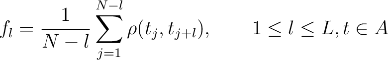
Where is the maximum lag value. Now, the first 20 features (one per amino acid in ) are
computed.
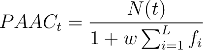
Where is the number of times the amino acid appears in the sequence, and is a
weighting factor set by default as 0.05, as suggested by Chou et al. (11).
Finally, the last set of features are added to the vector.
- Vector length
- Parameters
-
- –lag ,
default 30
- –weight ,
default 0.05
- –lag
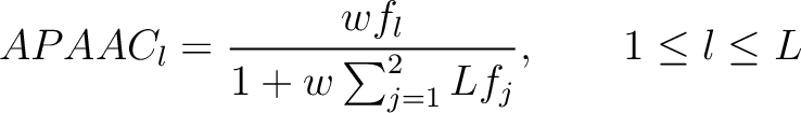
Amphiphilic Pseudo-Amino Acid Composition (APAAC)
The amphiphilic pseudo-amino acid composition method (25) only uses the
hydrophilicity () and hydrophobicity () values. These
values are used to define their correlation functions as:


Where is the group of the 20 natural amino acids. Now, the sequence-order can be found with
the following formula:
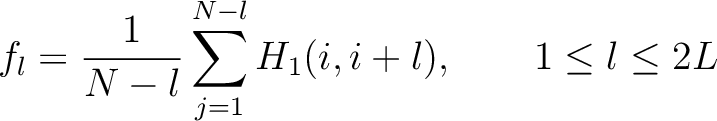
Where is the maximum lag value. Now, the first 20 features (one per amino acid in ) are
computed.
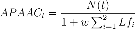
Where is the number of times the amino acid appears in the sequence, and is a
weighting factor set by default as 0.05, as suggested by Chou et al. (11).
Finally, the last set of features are added to the vector.
- Vector length
- Parameters
-
- –lag ,
default 30
- –weight ,
default 0.05
- –lag
Binary
Binary
The binary encoding (26) represents each amino acid in the sequence as a binary string of 20 numbers. For example, amino acid A is "10000000000000000000", C is "01000000000000000000", etc., following the order of "ACDEFGHIKLMNPQRSTVWY".
- Vector length
 , where is the sequence length
- Parameters None
- All sequences must have the same length
Taylor's Venn Diagram (TVD)
The Taylor's venn diagram method (27) is based on 10 physicochemical groups (hydrophobic, positive, negative, polar, charged, small, tiny, aliphatic, aromatic, proline) where the 20 natural amino acids might belong to. These amino acids are encoded as binary vectors of length 10 (1 per property), getting a 1 if the amino acid belonging to the group that has that property. For example, if the amino acid belongs to the hydrophobic group, it will get 1, and if not, it will get 0.
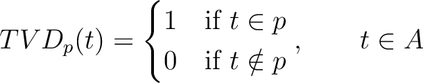
Where  is a property and is the set of the 20
natural amino acids. The full table with the binary values is found in Supplementary Material 2.
is a property and is the set of the 20
natural amino acids. The full table with the binary values is found in Supplementary Material 2.
- Vector length ,
where is the sequence length
- Parameters None
- All sequences must have the same length
Pseudo k-Tuple Reduced Amino Acid Composition (PseKRAAC)
The pseudo k-tuple reduced amino acid composition (28) represents proteins as
vectors that contain information based on K-tuples of reduced amino acid cluster (RAAC ) components. These
components can depend on a -
) components. These
components can depend on a - or a
or a  -
-
 , a type of reduced amino acid alphabet and a number of clusters (or mode).
These types and modes, as well as the groups, are found in Supplementary Material 2.
, a type of reduced amino acid alphabet and a number of clusters (or mode).
These types and modes, as well as the groups, are found in Supplementary Material 2.
For the - type of calculation, it represents the sequence-order information
of subsequences of length separated by residues. Thus, it
counts the number of times a combination of groups in the selected RAAC appears (Figure 2).
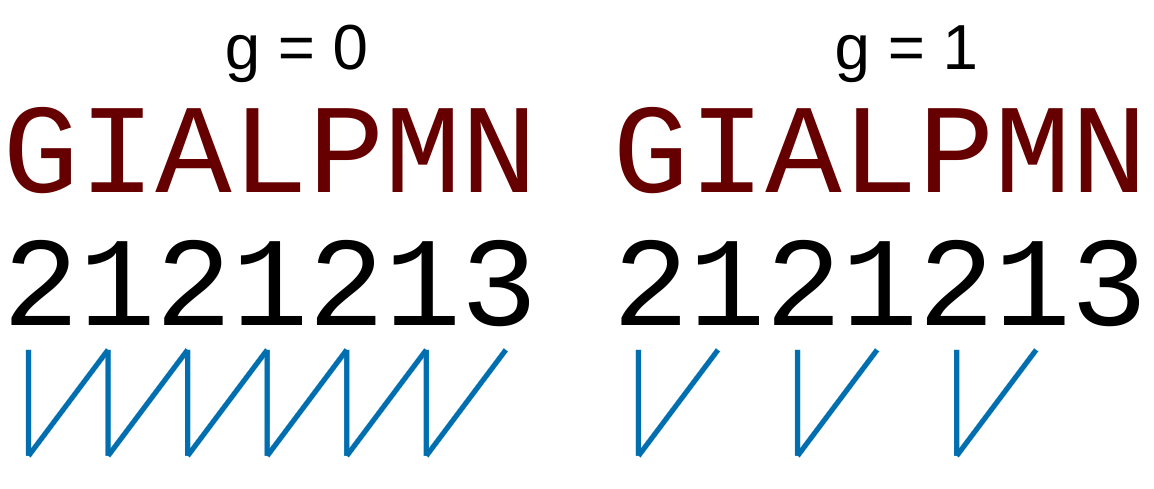 |
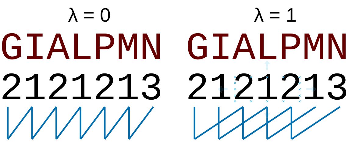
For the -
type of calculation, it represents the sequence-order information of groups
of amino acids separated by residues between amino acids. Thus, it counts the number of
times a combination of groups in the selected RAAC appears (Figure 3).
 |
- Vector length
- Parameters
-
- –type
 ,
required
,
required
- –raactype
 ,
required.
,
required.
- –subtype
 ,
required. g-gap or lambda-correlation
,
required. g-gap or lambda-correlation
- –ktuple , default
2. Can be 1, 2 or 3.
- –gapLambda
 , required. Value for or , depending on the subtype.
- –type
Secondary Structure with PSIPRED or SPINE-X
These encodings use the generated .ss2 files from PSIPRED (29) or the .spxOut files from SPINE-X (30). There must be one file per input sequence.
Secondary Structure Elements Binary (SSEB)
The secondary structure elements binary method (8) represents each amino acid, depending on the type of secondary structure element where they were classified in, as a vector of 3 binary digits. The elements are helix (001), sheet (010) and coil (100).
- Vector length
 , where is the sequence length
- Parameters
-
- –path, path where .ss2 and .spXout files are located. One per input sequence.
- All sequences must have the same length
Secondary Structure Elements Content (SSEC)
The secondary structure elements content method (8) calculates the frequency of each element type (helix, sheet, coil) found in the peptide sequence.
Where is the number of times the element appears in the
sequence, and is the sequence length
- Vector length 3
- Parameters
-
- –path, path where .ss2 and .spXout files are located. One per input sequence.
Secondary Structure Probabilities Bigram (SSPB)
Each amino acid in the sequence gets a probability of it having one of the three structural elements (helix,
coil, sheet). The secondary structure probabilities bigram (31) sums the
multiplication of the probabilities for each of the combinations between structural elements among the pairs of
amino acids separated by  residues. This parameter was added by us,
originally it was 1.
residues. This parameter was added by us,
originally it was 1.
Where  and
and
 are the probabilities of the amino acids at positions and
  in
the sequence having the elements and
in
the sequence having the elements and  , respectively, and
is
the sequence length.
, respectively, and
is
the sequence length.
- Vector length

- Parameters
-
- –path, path where .ss2 and .spXout files are located. One per input sequence.
- –n ,
default 1
Secondary Structure Probabilities Auto-Covariance (SSPAC)
Each amino acid in the sequence gets a probability of it having one of the three structural elements (helix,
coil, sheet). The secondary structure probabilities auto-covariance method (31) sums the multiplication of the probabilities for each structural element
among the pairs of amino acids separated by residues, where
ranges from 1 to .

Where and
 are the probabilities of the amino acids at positions and in
the sequence having the element , is the maximum value
for the separation between residues, and is the sequence
length.
are the probabilities of the amino acids at positions and in
the sequence having the element , is the maximum value
for the separation between residues, and is the sequence
length.
- Vector length
- Parameters
-
- –path, path where .ss2 and .spXout files are located. One per input sequence.
- –n , default
10
Secondary Structure with SPINE-X
These encodings use the generated .spxOut files from SPINE-X (30). There must be one file per input sequence.
Torsional Angles (TA)
The torsion angles method (8) adds the  and
and  values per amino acid to the vector.
- Vector length
 , where is the sequence length.
- Parameters
-
- –path, path where .spXout files are located. One per input sequence.
- All sequences must have the same length
Torsional Angles Composition (TAC)
The torsional angles composition (31) converts the and
values per amino acid from degrees to radians, calculates the sine and cosine of these two angles, divides these
values by the length of the sequence, and adds the 4 final values to the vector.
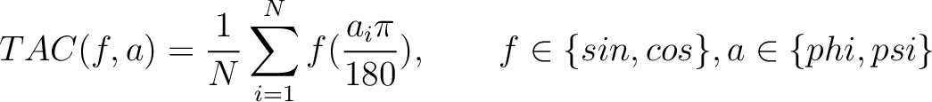
Where  is the or value for the
amino acid at position in the sequence, and is the sequence
length.
is the or value for the
amino acid at position in the sequence, and is the sequence
length.
- Vector length

- Parameters
-
- –path, path where .spXout files are located. One per input sequence.
Torsional Angles Bigram (TAB)
The torsional angles bigram (31) converts the and
values per amino acid from degrees to radians, and calculates the sine and cosine of these two angles, so each
amino acid has 4 associated values. Then, each type of value is multiplied as pairs in the sequence separated by
residues, and finally divided by the sequence length. This parameter was added by us,
originally it was 1.

Where and  are the or
values for the amino acid at position and in the sequence,
and
is the sequence length.
are the or
values for the amino acid at position and in the sequence,
and
is the sequence length.
- Vector length

- Parameters
-
- –path, path where .spXout files are located. One per input sequence.
- –n ,
default 1.
Torsional Angles Autocovariance (TAAC)
The torsional angles auto-covariance method (31) converts the and
values per amino acid from degrees to radians, and calculates the sine and cosine of these two angles, so each
amino acid has 4 associated values. Then, it sums the multiplication of each type of value among the pairs of
amino acids separated by residues, where ranges from 1 to
.

Where and are the or
values for the amino acid at position and in the sequence,
is
the maximum value for the separation between residues, and is the sequence
length.
- Vector length

- Parameters
-
- –path, path where .spXout files are located. One per input sequence.
- –n , default
10.
Accessible Surface Area (ASA)
The accessible surface area method (8) reads the ASA values per amino acid and adds them to the vector.
- Vector length ,
where is the sequence length.
- Parameters
-
- –path, path where .spXout files are located. One per input sequence.
- All sequences must have the same length
Disorder
The disorder-based methods use the generated .dis files generated by VSL2 (32). There must be one file per input sequence.
Disorder
The disorder method (33) reads the probability values per amino acid and adds them to the vector.
- Vector length ,
where is the sequence length.
- Parameters
-
- –path, path where .dis files are located. One per input sequence.
- All sequences must have the same length
Disorder Content (DisorderC)
The disorder content method (8) calculates the frequency of ordered and disordered residues in the sequence.
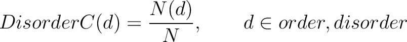
Where is the number of ordered or disordered residues in the sequence, and is the
sequence length.
- Vector length

- Parameters
-
- –path, path where .dis files are located. One per input sequence.
Disorder Binary (DisorderB)
The disorder binary method (8) encodes each amino acid as a binary vector of length 2. If the residue is ordered, then it is encoded as [1, 0], and if it is disordered, it is encoded as [0, 1].
- Vector length , where is the sequence length.
- Parameters
-
- –path, path where .dis files are located. One per input sequence.
- All sequences must have the same length
k-Nearest Neighbors
The k-nearest neighbors (KNN) methods require two additional files: a training file in FASTA format that will contain a training set, and a label file, which will contain the class each sequence corresponds to. The KNN method uses the similarity score between every two sequences in the training file as distance.
The
values depend on the total number of samples provided in the training file, finding the amount of sequences in
 of the training file. If the training file has 10 sequences,
then from 1% to 10% the value will be 1, from 11% to 20% the value will be 2, and so on.
of the training file. If the training file has 10 sequences,
then from 1% to 10% the value will be 1, from 11% to 20% the value will be 2, and so on.
k-Nearest Neighbors - Peptides (KNNpeptide)
The k-nearest neighbor for peptides method (34) indicates how many of the
sequences per each class in the neighboring % from the training
file are close to the input sequence according to the similarity score  , which is
calculated as:
, which is
calculated as:
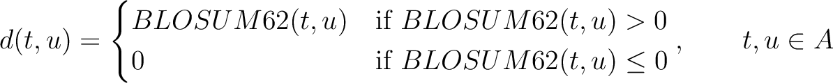
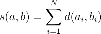
Where is the set of the 20 natural amino acids,
 is the value for the amino acid pair
  in the
BLOSUM62 matrix, and and
in the
BLOSUM62 matrix, and and  are the amino acids at position in the sequences
 and
and
 .
.
- Vector length
 , where
  is number of classes.
- Parameters
-
- –train, path where the fasta training file is located
- –labels, path where the label file is located. All sequences in the training file must be in the labels file.
- –k , default
30.
- All sequences must have the same length
k-Nearest Neighbors - Proteins (KNNproteins)
The k-nearest neighbor for proteins (8) indicates how many of the sequences per
each class in the neighboring k% from the training file are close to the input sequence, according to the
similarity score , which is calculated as:
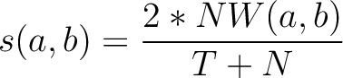
Where  is the number of equal characters in the resulting Needleman-Wunsch alignment
(35) between sequences and ,
is the number of equal characters in the resulting Needleman-Wunsch alignment
(35) between sequences and ,
 is
the number of training sequences, and is the sequence length.
is
the number of training sequences, and is the sequence length.
- Vector length , where is number of classes.
- Parameters
-
- –train, path where the fasta training file is located
- –labels, path where the label file is located. All sequences in the training file must be in the labels file.
- –k , default
30.
Position-Specific Scoring Matrix (PSSM)
The position-specific scoring matrix-based methods use the generated .pssm by blastpgp in legacy BLAST (36) and psiblast in BLAST+ (37) against the uniref50 database (38).
Position-Specific Scoring Matrix (PSSM)
The PSSM method (33) inserts all 20 values per sequence amino acid in the vector.
- Vector length , where is the sequence length.
- Parameters
-
- –path, path where the .pssm files are located. One per input sequence.
- All sequences must have the same length
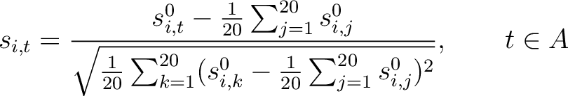
PSSM Amino Acid Composition (PSSMAAC)
The PSSM amino acid composition method (39) calculates the average score for each of the 20 natural amino acids along the whole sequence.
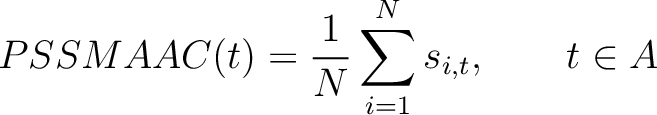
Where is the set of the 20 natural amino acids,  is the score
in the PSSM matrix for the amino acid at position in the sequence,
and
is the sequence length.
is the score
in the PSSM matrix for the amino acid at position in the sequence,
and
is the sequence length.
- Vector length
- Parameters
-
- –path, path where the .pssm files are located. One per input sequence.
Bigram PSSM (BiPSSM)
The bigram PSSM method (31) sums the product between the PSSM values of two
residues in the sequence separated by characters for two amino acid types and divides that sum by the
sequence length. This parameter was added by us, originally it was 1.
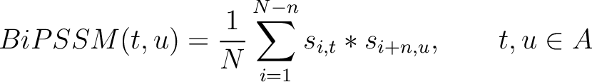
Where is the set of the 20 natural amino acids, and
 are the scores in the PSSM matrix for the amino acids and
  at
positions and respectively, and is the sequence
length.
at
positions and respectively, and is the sequence
length.
- Vector length
- Parameters
-
- –path, path where the .pssm files are located. One per input sequence.
- –n ,
default 1
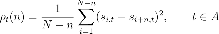
PSSM Autocovariance (PSSMAC)
The PSSM autocovariance method (40) calculates the autocovariance between two
residues separated by characters for a specific amino acid type.
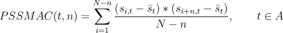
Where is the set of the 20 natural amino acids, and
 are the scores in the PSSM matrix for the amino acid at positions and
,
and
is the sequence length.
are the scores in the PSSM matrix for the amino acid at positions and
,
and
is the sequence length.
- Vector length
- Parameters
-
- –path, path where the .pssm files are located. One per input sequence.
- –n ,
default 1
Pseudo-PSSM (PPSSM)
The pseudo-PSSM method (41) finds the average for every amino acid type in the
PSSM matrix, and calculates the correlation between residues separated by characters per each
amino acid type. First, all values in the PSSM matrix must be standardized by using the following formula:
Where is the set of the 20 natural amino acids,
 is the initial score in the PSSM matrix for the amino acid at the
row , and
is the initial score in the PSSM matrix for the amino acid at the
row , and
 and
and
 are the initial scores in the PSSM matrix for the row , columns and
.
are the initial scores in the PSSM matrix for the row , columns and
.
Where and
are the standardized scores in the PSSM matrix for the amino acid at
rows and , and is the sequence
length.
The PPSSM vector is the concatenation of the 20 values for  and the 20
values of
and the 20
values of  .
.
- Vector length

- Parameters
-
- –path, path where the .pssm files are located. One per input sequence.
- –n ,
default 1
Other Encodings
Amino Acid Index (AAI)
The amino acid index method (42) uses the amino acid properties from the AAindex Database (14). This database has 544 different indices, where 531 have no "NA" values for any of the 20 amino acids. The features are the values for each amino acid in the sequence found in each one of the indices.
- Vector length
 , where is the sequence
length.
, where is the sequence
length.
- Parameters None
- All sequences must have the same length
BLOSUM62
The BLOSUM62 method (43) uses the BLOSUM62 matrix to get the features, which are all the values for the 20 amino acids in each respective row. This means that for every amino acid in the sequence there will be 20 features.
- Vector length , where is the sequence length.
- Parameters None
- All sequences must have the same length
Z-Scale (ZS)
The z-scale method (44) uses the z-scale table (45), where each amino acid type has 5 z-values. This means that for every amino acid in the sequence there will be 5 features.
- Vector length
 , where is the sequence length.
- Parameters None
- All sequences must have the same length
Bibliography
- 1
-
Manoj Bhasin and Gajendra P.S. Raghava.
Classification of Nuclear Receptors Based on Amino Acid Composition and Dipeptide Composition.
Journal of Biological Chemistry, 279(22):23262–23266, may 2004.
- 2
-
Ke Chen, Lukasz A. Kurgan, and Jishou Ruan.
Prediction of protein structural class using novel evolutionary collocation-based sequence representation.
Journal of Computational Chemistry, 29(10):1596–1604, jul 2008.
- 3
-
Vijayakumar Saravanan and Namasivayam Gautham.
Harnessing Computational Biology for Exact Linear B-Cell Epitope Prediction: A Novel Amino Acid Composition-Based Feature Descriptor.
OMICS: A Journal of Integrative Biology, 19(10):648–658, oct 2015.
- 4
-
J. Chen, H. Liu, J. Yang, and K.-C. Chou.
Prediction of linear B-cell epitopes using amino acid pair antigenicity scale.
Amino Acids, 33(3):423–428, sep 2007.
- 5
-
Sudipto Saha, Manoj Bhasin, and Gajendra PS Raghava.
Bcipep: A database of B-cell epitopes.
BMC Genomics, 6(1):79, dec 2005.
- 6
-
A. Bairoch.
The SWISS-PROT protein sequence database and its supplement TrEMBL in 2000.
Nucleic Acids Research, 28(1):45–48, jan 2000.
- 7
-
Jishou Ruan, Kui Wang, Jie Yang, Lukasz A. Kurgan, and Krzysztof Cios.
Highly accurate and consistent method for prediction of helix and strand content from primary protein sequences.
Artificial Intelligence in Medicine, 35(1-2):19–35, sep 2005.
- 8
-
Zhen Chen, Pei Zhao, Fuyi Li, André Leier, Tatiana T Marquez-Lago, Yanan
Wang, Geoffrey I Webb, A Ian Smith, Roger J Daly, Kuo-Chen Chou, and
Jiangning Song.
iFeature: a Python package and web server for features extraction and selection from protein and peptide sequences.
Bioinformatics, 34(14):2499–2502, jul 2018.
- 9
-
Tzong-Yi Lee, Zong-Qing Lin, Sheng-Jen Hsieh, Neil Arvin Bretaña, and
Cheng-Tsung Lu.
Exploiting maximal dependence decomposition to identify conserved motifs from a group of aligned signal sequences.
Bioinformatics, 27(13):1780–1787, jul 2011.
- 10
-
Zhen-Hui Zhang, Zheng-Hua Wang, Zhen-Rong Zhang, and Yong-Xian Wang.
A novel method for apoptosis protein subcellular localization prediction combining encoding based on grouped weight and support vector machine.
FEBS Letters, 580(26):6169–6174, nov 2006.
- 11
-
K C Chou.
Prediction of protein cellular attributes using pseudo-amino acid composition.
Proteins, 43(3):246–55, may 2001.
- 12
-
R. Grantham.
Amino Acid Difference Formula to Help Explain Protein Evolution.
Science, 185(4154):862–864, sep 1974.
- 13
-
G. Schneider and P. Wrede.
The rational design of amino acid sequences by artificial neural networks and simulated molecular evolution: de novo design of an idealized leader peptidase cleavage site.
Biophysical Journal, 66(2):335–344, feb 1994.
- 14
-
Shuichi Kawashima, Piotr Pokarowski, Maria Pokarowska, Andrzej Kolinski,
Toshiaki Katayama, and Minoru Kanehisa.
AAindex: amino acid index database, progress report 2008.
Nucleic acids research, 36(Database issue):D202–5, jan 2008.
- 15
-
Nan Xiao, Dong-Sheng Cao, Min-Feng Zhu, and Qing-Song Xu.
protr/ProtrWeb: R package and web server for generating various numerical representation schemes of protein sequences.
Bioinformatics (Oxford, England), 31(11):1857–9, jun 2015.
- 16
-
Robert R. Sokal and Barbara A. Thomson.
Population structure inferred by local spatial autocorrelation: An example from an Amerindian tribal population.
American Journal of Physical Anthropology, 129(1):121–131, jan 2006.
- 17
-
Z P Feng and C T Zhang.
Prediction of membrane protein types based on the hydrophobic index of amino acids.
Journal of protein chemistry, 19(4):269–75, may 2000.
- 18
-
David S. Horne.
Prediction of protein helix content from an autocorrelation analysis of sequence hydrophobicities.
Biopolymers, 27(3):451–477, mar 1988.
- 19
-
I. Dubchak, I. Muchnik, S. R. Holbrook, and S. H. Kim.
Prediction of protein folding class using global description of amino acid sequence.
Proceedings of the National Academy of Sciences, 92(19):8700–8704, sep 1995.
- 20
-
Inna Dubchak, Ilya Muchnik, Christopher Mayor, Igor Dralyuk, and Sung-Hou Kim.
Recognition of a protein fold in the context of the SCOP classification.
Proteins: Structure, Function, and Genetics, 35(4):401–407, jun 1999.
- 21
-
C.Z. Cai.
SVM-Prot: web-based support vector machine software for functional classification of a protein from its primary sequence.
Nucleic Acids Research, 31(13):3692–3697, jul 2003.
- 22
-
Juwen Shen, Jian Zhang, Xiaomin Luo, Weiliang Zhu, Kunqian Yu, Kaixian Chen,
Yixue Li, and Hualiang Jiang.
Predicting protein-protein interactions based only on sequences information.
Proceedings of the National Academy of Sciences of the United States of America, 104(11):4337–41, mar 2007.
- 23
-
Charles. Tanford.
Contribution of Hydrophobic Interactions to the Stability of the Globular Conformation of Proteins.
Journal of the American Chemical Society, 84(22):4240–4247, nov 1962.
- 24
-
T. P. Hopp and K. R. Woods.
Prediction of protein antigenic determinants from amino acid sequences.
Proceedings of the National Academy of Sciences, 78(6):3824–3828, jun 1981.
- 25
-
K.-C. Chou.
Using amphiphilic pseudo amino acid composition to predict enzyme subfamily classes.
Bioinformatics, 21(1):10–19, jan 2005.
- 26
-
Zhen Chen, Yong-Zi Chen, Xiao-Feng Wang, Chuan Wang, Ren-Xiang Yan, and Ziding
Zhang.
Prediction of Ubiquitination Sites by Using the Composition of k-Spaced Amino Acid Pairs.
PLoS ONE, 6(7):e22930, jul 2011.
- 27
-
William Ramsay Taylor.
The classification of amino acid conservation.
Journal of Theoretical Biology, 119(2):205–218, mar 1986.
- 28
-
Yongchun Zuo, Yuan Li, Yingli Chen, Guangpeng Li, Zhenhe Yan, and Lei Yang.
PseKRAAC: a flexible web server for generating pseudo K-tuple reduced amino acids composition.
Bioinformatics, 33(1):122–124, jan 2017.
- 29
-
David T. Jones.
Protein secondary structure prediction based on position-specific scoring matrices.
Journal of Molecular Biology, 292(2):195–202, 1999.
- 30
-
Eshel Faraggi, Tuo Zhang, Yuedong Yang, Lukasz Kurgan, and Yaoqi Zhou.
SPINE X: Improving protein secondary structure prediction by multistep learning coupled with prediction of solvent accessible surface area and backbone torsion angles.
Journal of Computational Chemistry, 33(3):259–267, jan 2012.
- 31
-
Farshid Rayhan, Sajid Ahmed, Swakkhar Shatabda, Dewan Md Farid, Zaynab
Mousavian, Abdollah Dehzangi, and M. Sohel Rahman.
iDTI-ESBoost: Identification of Drug Target Interaction Using Evolutionary and Structural Features with Boosting.
Scientific Reports, 7(1):17731, dec 2017.
- 32
-
Kang Peng, Predrag Radivojac, Slobodan Vucetic, A Keith Dunker, and Zoran
Obradovic.
Length-dependent prediction of protein intrinsic disorder.
BMC Bioinformatics, 7(1):208, dec 2006.
- 33
-
Yudong Cai, Tao Huang, Lele Hu, Xiaohe Shi, Lu Xie, and Yixue Li.
Prediction of lysine ubiquitination with mRMR feature selection and analysis.
Amino Acids, 42(4):1387–1395, apr 2012.
- 34
-
Xiang Chen, Jian Ding Qiu, Shao Ping Shi, Sheng Bao Suo, Shu Yun Huang, and
Ru Ping Liang.
Incorporating key position and amino acid residue features to identify general and species-specific Ubiquitin conjugation sites.
Bioinformatics, 29(13):1614–1622, 2013.
- 35
-
Saul B. Needleman and Christian D. Wunsch.
A general method applicable to the search for similarities in the amino acid sequence of two proteins.
Journal of Molecular Biology, 48(3):443–453, mar 1970.
- 36
-
S. Altschul.
Gapped BLAST and PSI-BLAST: a new generation of protein database search programs.
Nucleic Acids Research, 25(17):3389–3402, sep 1997.
- 37
-
Christiam Camacho, George Coulouris, Vahram Avagyan, Ning Ma, Jason
Papadopoulos, Kevin Bealer, and Thomas L Madden.
BLAST+: architecture and applications.
BMC Bioinformatics, 10(1):421, dec 2009.
- 38
-
B. E. Suzek, Y. Wang, H. Huang, P. B. McGarvey, and C. H. Wu.
UniRef clusters: a comprehensive and scalable alternative for improving sequence similarity searches.
Bioinformatics, 31(6):926–932, mar 2015.
- 39
-
Taigang Liu, Xiaoqi Zheng, and Jun Wang.
Prediction of protein structural class for low-similarity sequences using support vector machine and PSI-BLAST profile.
Biochimie, 92(10):1330–1334, oct 2010.
- 40
-
Qiwen Dong, Shuigeng Zhou, and Jihong Guan.
A new taxonomy-based protein fold recognition approach based on autocross-covariance transformation.
Bioinformatics, 25(20):2655–2662, oct 2009.
- 41
-
Hong Bin Shen and Kuo Chen Chou.
Nuc-PLoc: A new web-server for predicting protein subnuclear localization by fusing PseAA composition and PsePSSM.
Protein Engineering, Design and Selection, 20(11):561–567, 2007.
- 42
-
Chun-Wei Tung and Shinn-Ying Ho.
Computational identification of ubiquitylation sites from protein sequences.
BMC Bioinformatics, 9(1):310, dec 2008.
- 43
-
Tzong-Yi Lee, Shu-An Chen, Hsin-Yi Hung, and Yu-Yen Ou.
Incorporating Distant Sequence Features and Radial Basis Function Networks to Identify Ubiquitin Conjugation Sites.
PLoS ONE, 6(3):e17331, mar 2011.
- 44
-
Yong-Zi Chen, Zhen Chen, Yu-Ai Gong, and Guoguang Ying.
SUMOhydro: A Novel Method for the Prediction of Sumoylation Sites Based on Hydrophobic Properties.
PLoS ONE, 7(6):e39195, jun 2012.
- 45
-
Maria Sandberg, Lennart Eriksson, Jörgen Jonsson, Michael
Sjöström, and Svante Wold.
New Chemical Descriptors Relevant for the Design of Biologically Active Peptides. A Multivariate Characterization of 87 Amino Acids.
Journal of Medicinal Chemistry, 41(14):2481–2491, jul 1998.
About this document ...
This document was generated using the LaTeX2HTML translator Version 2020.2 (Released July 1, 2020)
The command line arguments were:
latex2html supp.tex -split 0
The translation was initiated on 2022-07-20